Attention: Everything You Need
Since Vaswani et al. dropped the Transformer paper in 2017, we've basically been optimizing the same few equations for nearly a decade. That elegant has spawned everything from GPT-4 to Llama to Claude—but getting from that formula to a system that actually serves millions of requests at reasonable cost is a different beast entirely.
This post is my attempt to go through the past decade. We'll move quickly through the fundamentals (you probably know them), then dig into what actually matters when you're trying to train on 100K token contexts or serve at scale without burning through your infrastructure budget.
Disclaimer: This post was written with the help of LLMs, with the content carefully curated based on papers I've read and systems I've used over the years. If you still notice any errors, please don't hesitate to send a note to [email protected].
What is Attention?
References: [1, 2]
Attention determines relevance. Given a query, which parts of the input matter? Scaled dot-product attention:
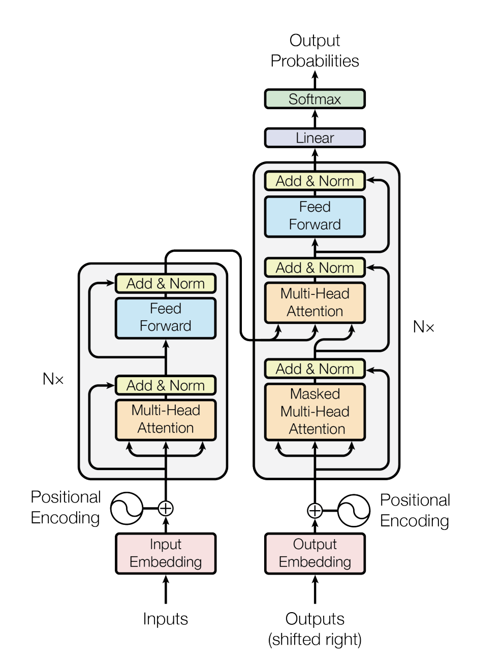 Figure 1: The Transformer model architecture showing multi-head attention and feed-forward layers. Source: Vaswani et al. (2017)
Three matrices:
- Query (Q): What we're looking for
- Key (K): What we're looking at
- Value (V): What we retrieve
Compute dot products between queries and keys for relevance scores, then weight the values accordingly.
The Scaling Factor
The scaling isn't arbitrary. Vaswani et al.: "We suspect that for large values of , the dot products grow large in magnitude, pushing the softmax function into regions where it has extremely small gradients".
If and contain i.i.d. elements with mean 0 and variance 1, their dot product has variance . Large dimensions → large dot products → softmax saturation → vanishing gradients.
Dividing by normalizes variance back to ~1. Gradients stay healthy, training stays stable.
Multi-Head Attention
References: [1, 2]
Single attention is useful, but multi-head attention is where things get interesting. Compute attention times in parallel, each with different learned projections:
where each head is:
Each head learns different weight matrices (, , ), focusing on different relationships. One head might capture subject-verb dependencies, another tracks long-range references, another focuses on syntactic patterns.
Multi-Head Design Benefits
Three advantages for production systems:
-
Embarrassingly Parallel: Each head computes independently—perfect for GPU acceleration and essential for production throughput.
-
Multiple Representational Subspaces: The original paper notes multi-head attention "allows the model to jointly attend to information from different representation subspaces at different positions". Different heads specialize in different phenomena simultaneously.
-
Robustness Through Redundancy: No single attention pattern required. Research shows certain heads can be pruned post-training without significant degradation, suggesting built-in redundancy.
What Attention Heads Learn
Research shows attention heads develop distinct patterns:
- Positional heads: Attend to adjacent tokens (position ) for local syntax
- Syntactic heads: Track grammatical relationships like subject-verb agreement
- Semantic heads: Capture long-range dependencies and coreference
- Rare heads: Focus on specific tokens like
[CLS],[SEP], punctuation
Tools like BertViz and Attention Flow let you inspect these patterns.
Studies show 10-20% of heads can be pruned with <1% quality loss—useful for model compression. Some heads are redundant, others critical.
Attention entropy as diagnostic: Low entropy (peaked) = focused on specific tokens. High entropy (uniform) = either not learning useful patterns or attending broadly.
The Permutation Equivariance Property
References: [3]
Here's a subtle but important property: multi-head attention is permutation-equivariant. If you swap input positions, outputs swap accordingly. Mathematically, for any permutation matrix :
This means the attention mechanism itself has no inherent bias toward position—it treats all positions equally. This is why positional encodings are necessary for sequence order. The mechanism is extremely flexible, but requires careful position encoding design (which led to innovations like RoPE and other alternatives).
Implementation Insights
References: [3, 4]
import torch
import torch.nn as nn

class ScaledDotProductAttention(nn.Module):
    def __init__(self, d_k, dropout=0.1):
        super().__init__()
        self.d_k = d_k
        self.dropout = nn.Dropout(dropout)

    def forward(self, Q, K, V, mask=None):
        scores = torch.matmul(Q, K.transpose(-2, -1)) / torch.sqrt(torch.tensor(self.d_k, dtype=torch.float32))

        if mask is not None:
            scores = scores.masked_fill(mask == 0, float('-inf'))

        attention_weights = torch.softmax(scores, dim=-1)

        # Dropout on attention weights, not output - forces learning redundant paths
        attention_weights = self.dropout(attention_weights)

        output = torch.matmul(attention_weights, V)

        return output, attention_weights
Attention dropout (typically ) is applied to attention weights after softmax. This prevents overfitting to specific attention patterns and encourages robustness. During training, it randomly zeros out some attention connections, forcing the model to learn multiple paths to each value.
class MultiHeadAttention(nn.Module):
    def __init__(self, d_model, num_heads):
        super().__init__()
        assert d_model % num_heads == 0, "d_model must be divisible by num_heads"

        self.d_model = d_model
        self.num_heads = num_heads
        self.d_k = d_model // num_heads

        self.W_q = nn.Linear(d_model, d_model)
        self.W_k = nn.Linear(d_model, d_model)
        self.W_v = nn.Linear(d_model, d_model)
        self.W_o = nn.Linear(d_model, d_model)

        self.attention = ScaledDotProductAttention(self.d_k)

    def split_heads(self, x, batch_size):
        x = x.view(batch_size, -1, self.num_heads, self.d_k)
        return x.transpose(1, 2)

    def forward(self, Q, K, V, mask=None):
        batch_size = Q.size(0)

        Q = self.W_q(Q)
        K = self.W_k(K)
        V = self.W_v(V)

        Q = self.split_heads(Q, batch_size)
        K = self.split_heads(K, batch_size)
        V = self.split_heads(V, batch_size)

        attn_output, attn_weights = self.attention(Q, K, V, mask)

        # .contiguous() required before view() after transpose - triggers memory copy
        attn_output = attn_output.transpose(1, 2).contiguous()
        attn_output = attn_output.view(batch_size, -1, self.d_model)

        output = self.W_o(attn_output)

        return output, attn_weights
This implementation makes the parallel structure explicit—each head operates independently before concatenation.
Cross-Attention vs Self-Attention
References: [1]
While self-attention relates positions within a single sequence, cross-attention relates positions between two different sequences. This is fundamental for many architectures:
In self-attention: , , all come from the same sequence In cross-attention: comes from one sequence (target), and come from another (source)
class CrossAttention(nn.Module):
    def __init__(self, d_model, num_heads):
        super().__init__()
        self.num_heads = num_heads
        self.d_k = d_model // num_heads
        self.d_model = d_model

        self.W_q = nn.Linear(d_model, d_model)
        self.W_k = nn.Linear(d_model, d_model)
        self.W_v = nn.Linear(d_model, d_model)
        self.W_o = nn.Linear(d_model, d_model)

    def forward(self, target, source, mask=None):
        batch_size = target.size(0)

        # Q from target, K/V from source - this is the key difference
        Q = self.W_q(target)
        K = self.W_k(source)
        V = self.W_v(source)

        Q = Q.view(batch_size, -1, self.num_heads, self.d_k).transpose(1, 2)
        K = K.view(batch_size, -1, self.num_heads, self.d_k).transpose(1, 2)
        V = V.view(batch_size, -1, self.num_heads, self.d_k).transpose(1, 2)

        scores = torch.matmul(Q, K.transpose(-2, -1)) / math.sqrt(self.d_k)
        if mask is not None:
            scores = scores.masked_fill(mask == 0, float('-inf'))
        attention = torch.softmax(scores, dim=-1)
        output = torch.matmul(attention, V)

        output = output.transpose(1, 2).contiguous()
        output = output.view(batch_size, -1, self.d_model)

        return self.W_o(output)
Applications:
- Machine translation: Decoder attends to encoder outputs (T5, BART)
- Vision-language models: Text attends to image patches (CLIP, Flamingo)
- Speech-to-speech: Target speech attends to source speech features
- Retrieval-augmented generation: Query attends to retrieved documents
The Transformer architecture uses both: self-attention in encoder and decoder, plus cross-attention connecting them.
Causal Attention: Preventing Information Leakage
References: [1]
Autoregressive models like GPT and Llama must generate tokens sequentially—each token can only depend on previous tokens, not future ones. Causal masking (also called autoregressive or look-ahead masking) enforces this constraint:
This ensures token can only attend to positions . The mask is applied before softmax, setting future positions to so they have zero weight after softmax:
def create_causal_mask(seq_len):
    # Upper triangle masks positions j > i
    mask = torch.triu(torch.ones(seq_len, seq_len), diagonal=1).bool()
    return mask

def causal_attention(Q, K, V):
    d_k = Q.size(-1)
    scores = torch.matmul(Q, K.transpose(-2, -1)) / math.sqrt(d_k)

    # Mask applied BEFORE softmax - sets future to -inf
    mask = create_causal_mask(Q.size(-2)).to(Q.device)
    scores = scores.masked_fill(mask, float('-inf'))

    attention_weights = torch.softmax(scores, dim=-1)
    output = torch.matmul(attention_weights, V)
    return output
In production:
- Training: Can parallelize across sequence (teacher forcing with causal mask)
- Inference: Must generate token-by-token (autoregressive), cannot parallelize
- KV caching: Essential for efficient inference—cache previous tokens' K, V to avoid recomputation
Bidirectional vs Causal:
- BERT uses bidirectional attention (no mask) for understanding tasks
- GPT uses causal attention for generation tasks
- Encoder-decoder models use both: bidirectional in encoder, causal in decoder
Memory & Compute Optimizations
References: [5, 13, 14]
Modern transformer training faces significant memory bottlenecks. The following techniques address these challenges to enable efficient training at scale.
Mixed Precision Training: Foundation for Efficiency
Before diving into attention-specific optimizations, mixed precision training (FP16/BF16) is the foundational technique that enables all other optimizations. Instead of using 32-bit floating point (FP32) for all computations, mixed precision uses 16-bit formats for most operations while maintaining FP32 for critical accumulations.
Two main formats:
- FP16 (Float16): Standard half precision, 2x memory savings, but prone to underflow/overflow
- BF16 (BFloat16): Same range as FP32 but lower precision, preferred for stability
BF16 advantages:
- Same dynamic range as FP32 (8-bit exponent) reduces underflow/overflow compared to FP16
- No loss scaling required (unlike FP16)—the main practical benefit
- Native hardware support on A100, H100, and newer GPUs
- Pairs perfectly with FlashAttention and other optimizations
- 2x memory savings (enables 2x larger batch sizes or longer sequences)
- 2-3x training speedup from faster compute on Tensor Cores
- Minimal quality degradation (<0.1% on most benchmarks)
# PyTorch automatic mixed precision
from torch.cuda.amp import autocast, GradScaler

# BF16 training (preferred - no loss scaling needed)
with autocast(dtype=torch.bfloat16):
    output = model(input)
    loss = criterion(output, target)

# FP16 training (requires loss scaling to prevent underflow)
scaler = GradScaler()
with autocast(dtype=torch.float16):
    output = model(input)
    loss = criterion(output, target)
scaler.scale(loss).backward()
scaler.step(optimizer)
scaler.update()
Mixed precision is now standard in all production training pipelines—it's the first optimization to enable, not an optional extra.
The Next Frontier: FP8 Training
References: [19, 20]
Modern hardware (NVIDIA H100/B200) natively supports FP8 (8-bit floating point), doubling throughput over BF16. FP8 uses two formats: E4M3 (higher precision) for forward pass, E5M2 (wider range) for gradients.
Libraries like NVIDIA's Transformer Engine handle FP8 automatically with delayed scaling. For inference, FP8 is gaining ground for Llama-4 class models—2x faster weight loading than BF16 without INT4's quantization noise. Note that INT8 inference remains more common in production as of 2026, but FP8 is rapidly gaining adoption on newer hardware.
Trade-off: Requires H100+ hardware. BF16 remains the safer default, but FP8 is the future for cutting-edge systems.
FlashAttention: The I/O Revolution
Understanding attention's computational complexity is one thing; understanding its memory access patterns is another. The real bottleneck in modern hardware isn't compute—it's memory bandwidth.
Important distinction: FlashAttention reduces memory usage from to by not materializing the full attention matrix, while maintaining computational complexity (FLOPs). The 2-4x speedup comes from optimizing memory I/O between HBM and SRAM, not from reducing arithmetic operations. This is a common misconception worth clarifying.
FlashAttention reformulates attention to minimize memory reads and writes between GPU high-bandwidth memory (HBM) and on-chip SRAM. Key insight: instead of materializing the full attention matrix in HBM, compute attention in blocks that fit in SRAM, using tiling and recomputation strategies.
The Memory Hierarchy Problem
Modern GPUs have a memory hierarchy:
- HBM (High-Bandwidth Memory): Large (40GB+) but slow (~1.5 TB/s)
- SRAM (On-chip memory): Small (~20MB) but fast (~19 TB/s)
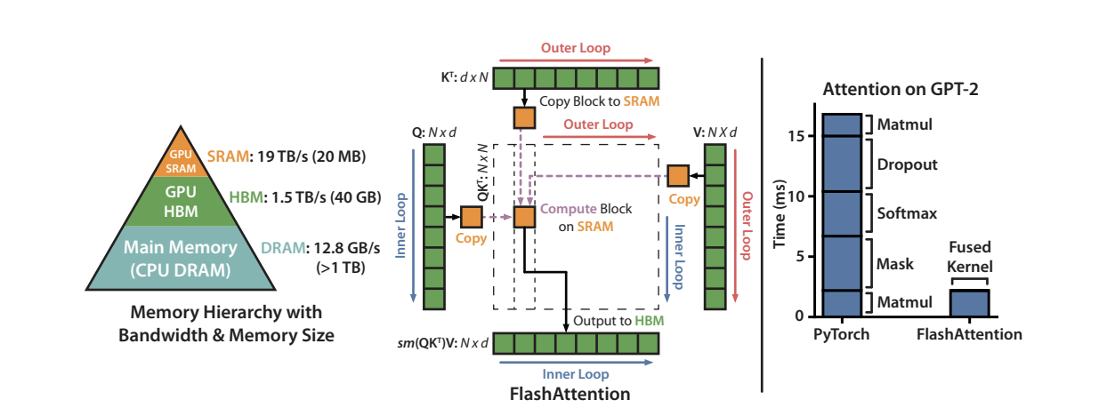 Figure 2: GPU memory hierarchy showing the speed-capacity tradeoff between HBM and SRAM. FlashAttention optimizes data movement between these levels. Source: Dao et al. (2022)
Standard attention implementations:
- Load , from HBM → compute → write to HBM
- Load from HBM → compute softmax → write to HBM
- Load softmax output and from HBM → compute final output
Each step involves expensive HBM reads/writes. For a sequence of length 4096 with hidden dimension 1024, the attention matrix alone requires 64MB—larger than SRAM capacity.
FlashAttention's Solution
FlashAttention uses tiling and kernel fusiont:
- Tiling: Split , , into blocks that fit in SRAM
- Online Softmax: Compute softmax incrementally without materializing the full attention matrix
- Recomputation: In the backward pass, recompute attention on-the-fly rather than storing it
Result: 2-4x speedups and the ability to handle much longer sequences. This isn't just an optimization—it's what makes training on sequences of 16K+ tokens practical.
# Conceptual pseudocode for FlashAttention's forward pass
def flash_attention_forward(Q, K, V, block_size):
    O = zeros_like(Q)
    l = zeros(Q.shape[0])
    m = full(Q.shape[0], -inf)

    for k_block, v_block in blocks(K, V, block_size):
        for q_block in blocks(Q, block_size):
            q_sram = load_to_sram(q_block)
            k_sram = load_to_sram(k_block)
            v_sram = load_to_sram(v_block)

            scores = q_sram @ k_sram.T / sqrt(d_k)

            # Online softmax - incrementally update statistics
            m_old, l_old = m, l
            m_new = max(m_old, max(scores))
            l_new = exp(m_old - m_new) * l_old + sum(exp(scores - m_new))

            # Rescale old output and add new contribution
            O_scaled = exp(m_old - m_new) * O
            new_contribution = exp(scores - m_new) @ v_sram
            O = (l_old * O_scaled + new_contribution) / l_new

            m, l = m_new, l_new

    return O
By recomputing attention during backpropagation rather than storing it, FlashAttention trades minimal extra compute for massive memory savings—a favorable tradeoff since modern GPUs are compute-rich but memory-bound.
FlashAttention-2 and FlashAttention-3
FlashAttention-2 improved upon FA-1 by changing the parallelization strategy to reduce non-matmul FLOPs and improve GPU occupancy. FA-1's inner loop over K blocks was sequential, limiting parallelization. FA-2 reorganized work partitioning across threads—each warp handles contiguous rows, reducing shared memory bank conflicts and enabling better coalesced memory access. By minimizing rescaling operations and fusing softmax with matmul operations more efficiently, FA-2 achieved ~2x speedup over FA-1, especially on A100 GPUs.
FlashAttention-3 targets H100's new architectural features: Tensor Memory Accelerator (TMA) for asynchronous memory transfers, Warp Group Matrix-Multiply-Accumulate (WGMMA) for cooperative matmuls, and asynchronous pipelines. FA-3 introduces warp specialization—producer warps handle memory operations while consumer warps focus on compute, overlapping three stages (load, compute, write) concurrently on different data. This software pipelining maximizes GPU utilization, achieving 1.5-2x speedup for FP16 and 2-3x for FP8 (with H100's native FP8 support) compared to FA-2, especially impactful for long sequences (8K-16K+). The evolution from FA-1 → FA-2 → FA-3 demonstrates how algorithms must co-evolve with hardware for optimal performance.
Gradient Checkpointing: Trading Compute for Memory
Core Idea: During backpropagation, recompute intermediate activations on-demand instead of storing them all in memory.
Standard backpropagation:
- Forward: Compute and store ALL intermediate activations (attention scores, FFN activations, dropout masks, layer outputs)
- Backward: Use stored activations to compute gradients
- Memory: where = num_layers, = seq_len, = hidden_dim
With checkpointing:
- Forward: Only save inputs to checkpointed segments, discard internal activations
- Backward: Recompute activations from saved checkpoints when needed
- Memory: with optimal checkpointing, or if checkpointing every layer
import torch.utils.checkpoint as checkpoint

class CheckpointedTransformerLayer(nn.Module):
    def forward(self, x, position_ids):
        return checkpoint.checkpoint(
            self._forward_impl,
            x, position_ids,
            use_reentrant=False  # Safer, modern approach
        )

    def _forward_impl(self, x, position_ids):
        # Internal activations discarded after forward
        x = x + self.attention(self.norm1(x), position_ids)
        x = x + self.ffn(self.norm2(x))
        return x
Tradeoffs:
- Memory reduction: 60-80% for large models
- Speed cost: 20-30% slower (forward pass runs twice per layer)
- Gradient quality: Mathematically identical to standard backprop
When to use: Training large models that don't fit in GPU memory, maximizing batch size or sequence length.
When NOT to use: Inference (no backprop), when memory isn't the bottleneck.
Combined techniques: FlashAttention + checkpointing enables 10x+ longer sequences. Works well with mixed precision and ZeRO optimizer for massive models.
In production, inference latency and throughput directly impact user experience and cost.
Inference Optimizations
References: [6, 7, 8, 9, 10, 16]
Modern LLMs face unique challenges during inference—particularly around memory efficiency and latency. The following techniques address these bottlenecks to enable fast, cost-effective serving at scale.
Grouped Query Attention (GQA): The KV Cache Solution
During autoregressive generation, models cache key-value pairs from previous tokens to avoid recomputation. For a model with 32 attention heads and 128-dimensional head size, each token requires storing values per token. At 100K context length, this becomes approximately 819M values per layer—a massive memory bottleneck.
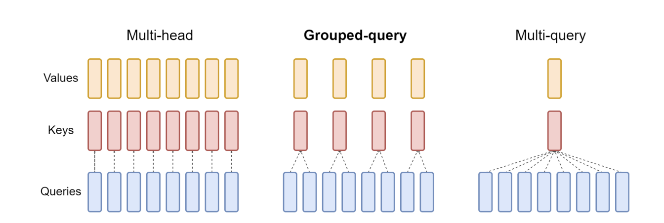 Figure 3: Comparison of Multi-Head Attention (MHA), Multi-Query Attention (MQA), and Grouped Query Attention (GQA). GQA groups query heads to share KV heads, balancing quality and efficiency. Source: Ainslie et al. (2023)
Multi-Query Attention (MQA) proposed a radical solution: share a single key-value head across all query heads. This reduces KV cache by 32x but comes with potential quality degradation (~1-2% on benchmarks), which can be largely mitigated through uptraining (continuing training with MQA architecture).
Grouped Query Attention (GQA) found the sweet spot. Instead of 32 separate KV heads (MHA) or 1 shared KV head (MQA), use 8 KV heads with 4 query heads per group:
class GroupedQueryAttention(nn.Module):
    def __init__(self, d_model, num_query_heads, num_kv_heads):
        super().__init__()
        assert num_query_heads % num_kv_heads == 0

        self.num_query_heads = num_query_heads
        self.num_kv_heads = num_kv_heads
        self.num_queries_per_kv = num_query_heads // num_kv_heads
        self.d_k = d_model // num_query_heads

        self.W_q = nn.Linear(d_model, num_query_heads * self.d_k)
        self.W_k = nn.Linear(d_model, num_kv_heads * self.d_k)
        self.W_v = nn.Linear(d_model, num_kv_heads * self.d_k)
        self.W_o = nn.Linear(d_model, d_model)

    def forward(self, x):
        batch_size, seq_len, _ = x.shape

        Q = self.W_q(x).view(batch_size, seq_len, self.num_query_heads, self.d_k)
        K = self.W_k(x).view(batch_size, seq_len, self.num_kv_heads, self.d_k)
        V = self.W_v(x).view(batch_size, seq_len, self.num_kv_heads, self.d_k)

        # repeat_interleave copies memory - production uses expand() or custom kernels
        K = K.repeat_interleave(self.num_queries_per_kv, dim=2)
        V = V.repeat_interleave(self.num_queries_per_kv, dim=2)

        scores = torch.matmul(Q, K.transpose(-2, -1)) / math.sqrt(self.d_k)
        attn_weights = torch.softmax(scores, dim=-1)
        output = torch.matmul(attn_weights, V)

        output = output.transpose(1, 2).contiguous().view(batch_size, seq_len, -1)
        return self.W_o(output)
The results are remarkable: 4x reduction in KV cache size with minimal quality loss (<0.1% on most benchmarks). Llama-2, Mistral, and Gemma all use GQA. Even better, existing MHA models can be "uptrained" to GQA using only 5% of original training compute.
Multi-Head Latent Attention (MLA): Extreme Compression
References: [17, 18]
While GQA reduces memory by sharing KV heads, Multi-Head Latent Attention (MLA)—introduced in DeepSeek-V2 and refined in DeepSeek-V3—takes a more aggressive approach: low-rank key-value joint compression.
Instead of storing full Key and Value matrices (even shared ones), MLA projects them into a low-dimensional latent vector during inference.
The mechanism:
- Compression: Inputs are projected down to a small latent dimension (e.g., 512) using a down-projection matrix
- Storage: Only this tiny compressed latent vector is stored in the KV cache, drastically reducing memory footprint
- Decompression: During attention computation, the latent vector is up-projected using and to generate the full heads on-the-fly
- Decoupled RoPE: To prevent positional information from interfering with compression, MLA uses a separate "pe" (positional embedding) vector that bypasses the compression bottleneck
class MultiHeadLatentAttention(nn.Module):
    def __init__(self, d_model, num_heads, d_latent, rope_dim):
        super().__init__()
        self.num_heads = num_heads
        self.head_dim = d_model // num_heads

        self.w_dkv = nn.Linear(d_model, d_latent, bias=False)

        self.w_uk = nn.Linear(d_latent, num_heads * self.head_dim, bias=False)
        self.w_uv = nn.Linear(d_latent, num_heads * self.head_dim, bias=False)

        self.w_kr = nn.Linear(d_model, rope_dim, bias=False)

    def forward(self, x, position_ids):
        c_kv = self.w_dkv(x)

        k = self.w_uk(c_kv)
        v = self.w_uv(c_kv)

        k_rope = apply_rope(self.w_kr(x), position_ids)
        k = torch.cat([k, k_rope], dim=-1)

        return k, v
Impact: MLA enables extreme KV cache compression—models with massive head counts (e.g., 128 heads) achieve KV cache sizes smaller than even GQA models, often compressing memory usage by 90%+ compared to standard MHA.
Real-world deployment: This breakthrough is why DeepSeek-V3 can efficiently serve a 671B parameter model at production scale. By compressing the KV cache to a fraction of what GQA would require, MLA makes serving massive MoE models economically viable—a critical enabler for the next generation of ultra-large language models.
Adoption note: As of 2026, MLA remains primarily a DeepSeek innovation (V2 and V3) and has not yet been widely adopted by other model families. Most production systems still use GQA as the standard KV cache optimization.
Beyond GQA: KV Cache Compression
While GQA reduces cache size through architectural changes, additional compression techniques push efficiency further:
- Quantization: Store KV cache in 8-bit or 4-bit precision instead of 16-bit (2-4x savings with minimal quality loss)
- Eviction policies: Drop least-important cached tokens based on attention scores
- Streaming LLMs: Keep only recent tokens plus "attention sinks" (initial tokens that accumulate disproportionate attention)
- H2O (Heavy Hitters Oracle): Cache only high-attention tokens, evict low-attention ones
Example impact: Combining INT8 quantization with GQA reduces cache from 32GB → 2GB for a 70B parameter model at 4K context.
Attention sinks: Initial tokens accumulate disproportionate attention weight even when semantically irrelevant. Keeping these tokens in cache is critical for long-context generation quality—evicting them causes catastrophic degradation.
Rotary Position Embedding (RoPE): Encoding Position Elegantly
Remember the permutation equivariance property? We need positional information, but how we encode it matters enormously. The original Transformer used learned absolute position embeddings. RoPE took a different approach: encode position by rotating query and key vectors in high-dimensional space.
Key insight: if we rotate by angle and by angle , their dot product naturally depends on the relative distance :
In practice, this complex rotation is implemented using sine and cosine operations on real-valued vectors. There are two common implementation variants:
Interleaved (Llama-style): Rotates adjacent pairs of features :
Rotary Half (GPT-NeoX/PaLM): Splits the vector into two halves and rotates them against each other:
where for the -th dimension pair.
Critical: Both variants are mathematically valid and produce equivalent relative position encoding, but they are incompatible when loading pre-trained weights. Llama models expect interleaved, while GPT-NeoX/PaLM expect rotary half. Using the wrong variant will produce garbage outputs.
def apply_rotary_pos_emb(q, k, position_ids):
    """Rotary Half variant (GPT-NeoX/PaLM style).

    WARNING: This implements the 'Rotary Half' variant which splits the vector
    into two halves. Llama models use the 'Interleaved' variant which rotates
    adjacent pairs. Both are mathematically valid but INCOMPATIBLE when loading
    pre-trained weights. Always verify which variant your model expects!
    """
    def rotate_half(x):
        # Split into first half and second half
        x1 = x[..., :x.shape[-1] // 2]
        x2 = x[..., x.shape[-1] // 2:]
        # Rotate: (-x2, x1) implements the 90-degree rotation
        return torch.cat((-x2, x1), dim=-1)

    seq_len = position_ids.shape[1]
    d_model = q.shape[-1]
    device = q.device

    inv_freq = 1.0 / (10000 ** (torch.arange(0, d_model, 2).float().to(device) / d_model))
    freqs = torch.outer(position_ids.float(), inv_freq)
    emb = torch.cat((freqs, freqs), dim=-1)

    cos = emb.cos()
    sin = emb.sin()

    q_embed = (q * cos) + (rotate_half(q) * sin)
    k_embed = (k * cos) + (rotate_half(k) * sin)

    return q_embed, k_embed
Note: In practice, libraries like Hugging Face Transformers handle RoPE implementation automatically and correctly for each model architecture. The code above is for educational purposes—you typically don't need to implement this yourself.
RoPE advantages:
- Zero parameters: No learned embeddings to store
- Inherently relative: Attention depends on relative distance, not absolute position
- Extrapolation: Can handle sequences longer than training length with proper scaling
- Universal adoption: Llama, GPT-NeoX, PaLM, Mistral all use RoPE
For extending to ultra-long contexts (100K+ tokens), techniques like linear interpolation, NTK-aware scaling, and YaRN modify the frequency base to maintain performance.
ALiBi: Simpler Position Encoding
An alternative to RoPE is ALiBi (Attention with Linear Biases), which adds position-dependent bias directly to attention scores:
where is a head-specific slope (e.g., for head ).
Even simpler than RoPE:
- No position embeddings to compute or apply
- Just subtract distance penalty from attention scores
- Used in: BLOOM, MPT models
Trade-off: RoPE provides slightly better quality on most benchmarks, but ALiBi offers simpler implementation and competitive performance. The choice often depends on engineering constraints and specific use cases.
PagedAttention: Virtual Memory for KV Cache
Even with GQA reducing cache size, managing memory efficiently during inference remains challenging. Consider serving multiple requests with varying sequence lengths—traditional approaches pre-allocate maximum memory per request, leading to ~60% memory waste from fragmentation.
PagedAttention, implemented in the vLLM serving framework, applies operating system virtual memory concepts to KV cache management. Instead of contiguous memory allocation, it stores KV cache in fixed-size blocks (e.g., 16 tokens) with a logical-to-physical mapping:
# Conceptual PagedAttention structure
class PagedKVCache:
    def __init__(self, block_size=16, num_blocks=1000):
        self.block_size = block_size
        # Physical memory: pre-allocated blocks
        self.physical_blocks = torch.zeros(num_blocks, block_size, d_model)
        self.free_blocks = list(range(num_blocks))

        # Logical to physical mapping per sequence
        self.block_tables = {}  # seq_id -> [physical_block_ids]

    def allocate_sequence(self, seq_id, num_tokens):
        """Allocate blocks for a new sequence"""
        num_blocks_needed = (num_tokens + self.block_size - 1) // self.block_size
        allocated = [self.free_blocks.pop() for _ in range(num_blocks_needed)]
        self.block_tables[seq_id] = allocated
        return allocated

    def append_tokens(self, seq_id, kv_data):
        """Append new tokens to sequence cache"""
        blocks = self.block_tables[seq_id]
        # Write to physical blocks via mapping
        # If current block is full, allocate new block
        if self._is_block_full(blocks[-1]):
            new_block = self.free_blocks.pop()
            blocks.append(new_block)

        self._write_to_block(blocks[-1], kv_data)

    def share_prefix(self, seq_id_1, seq_id_2, prefix_length):
        """Share common prefix blocks between sequences (for beam search)"""
        prefix_blocks = prefix_length // self.block_size
        # Both sequences point to same physical blocks for prefix
        shared = self.block_tables[seq_id_1][:prefix_blocks]
        self.block_tables[seq_id_2] = shared + self._allocate_new_blocks(...)
Advantages:
- Dynamic allocation: Allocate memory as sequences grow
- Memory sharing: Multiple sequences can share prefix blocks (critical for beam search)
- Defragmentation: Move blocks to consolidate free space
- Continuous batching: Efficiently batch requests of different lengths
Result: 2-4x higher throughput than alternatives, reducing memory waste from ~60% to ~20%. vLLM has become the de facto standard for LLM serving.
Continuous Batching: Maximizing GPU Utilization
Traditional batching waits for all requests in a batch to complete before starting new ones:
Batch 1: [Request A (1000 tokens), Request B (100 tokens), Request C (500 tokens)]
→ Wait for A (1000 tokens) to finish before starting Batch 2
→ GPU idle waiting for longest request
Continuous batching (Orca, implemented in vLLM) adds new requests as soon as capacity is available:
class ContinuousBatcher:
    def __init__(self, max_batch_size, max_tokens):
        self.running_requests = []
        self.waiting_queue = []

    def step(self):
        # Generate one token for each running request
        for req in self.running_requests:
            token = model.generate_next_token(req)
            req.append(token)

            # Remove completed requests
            if req.is_complete():
                self.running_requests.remove(req)

        # Fill available capacity with waiting requests
        while (len(self.running_requests) < self.max_batch_size and
               self.waiting_queue):
            new_req = self.waiting_queue.pop(0)
            self.running_requests.append(new_req)
Advantages:
- Near-100% GPU utilization vs ~60% with static batching
- Lower latency for short requests (don't wait for long requests)
- Better throughput overall
Enabler: PagedAttention's non-contiguous memory allocation allows mixing requests at different generation stages.
Speculative Decoding: Accelerating Inference 2-3x
Autoregressive generation is inherently sequential—each token requires a full model forward pass. Speculative Decoding achieves 2-3x speedup without changing outputs or retraining by using a small "draft" model to predict multiple tokens, then verifying them in parallel with the target model.
Core insight: Language modeling tasks often contain easier subtasks. A small, fast model can draft plausible continuations, and the large model can verify multiple candidates in a single forward pass.
Algorithm:
- Draft phase: Small model generates candidate tokens (fast, lower quality)
- Verification phase: Large model processes all candidates in parallel (single forward pass)
- Acceptance: Accept tokens where draft and target distributions agree
- Rejection sampling: Use modified rejection sampling to maintain exact target distribution
def speculative_decode(target_model, draft_model, prompt, k=4):
    """Speculative decoding maintains exact target distribution

    Note: This is a simplified version. Production implementations
    use modified rejection sampling to maintain exact distribution.
    See Leviathan et al. (2023) for complete algorithm.
    """
    tokens = prompt

    while not done:
        # Draft: small model generates k candidates (10-100x faster)
        draft_tokens = draft_model.generate(tokens, num_tokens=k)

        # Verify: target model scores all candidates in parallel
        target_probs = target_model.forward(tokens + draft_tokens)
        draft_probs = draft_model.forward(tokens + draft_tokens)

        # Accept/reject with modified rejection sampling
        for i in range(k):
            p_target = target_probs[i]
            p_draft = draft_probs[i]

            # Accept if draft probability ≥ target (common case)
            if random.random() < min(1, p_target / p_draft):
                tokens.append(draft_tokens[i])
            else:
                # Reject: sample from adjusted distribution (renormalize before sampling)
                adjusted_prob = max(0, p_target - p_draft)
                tokens.append(sample_from(adjusted_prob))
                break  # Stop at first rejection

    return tokens
How this works:
- Draft model is 10-100x faster (smaller, quantized, or distilled)
- Even 50% acceptance rate gives 2x speedup (process multiple tokens per target pass)
- Mathematically guaranteed to match target model's distribution exactly
- No retraining or architecture changes required
Production adoption: Google PaLM (2-3x speedup), Meta Llama serving, Medusa (multiple draft heads), and various inference frameworks. Works best when:
- Draft model is 10x+ faster than target
- Acceptance rate > 60% (predictable text, code, structured output)
- Batch size is small (latency-sensitive applications)
Trade-offs: Less effective for creative/unpredictable generation where draft model struggles to match target distribution.
Prompt Caching: Eliminating Redundant Computation
Many LLM requests share common prefixes—system prompts, few-shot examples, or document context. Prompt caching (prefix caching, KV cache reuse) eliminates redundant computation by caching and reusing KV pairs from identical prefixes.
How it works:
- Compute KV cache for prompt prefix during first request
- Store cached KV pairs with hash of prefix tokens
- For subsequent requests with same prefix, load cached KV and only compute new tokens
- Cache expires after 5 minutes of inactivity (Anthropic) or uses LRU eviction
Example scenario:
Request 1: [System Prompt (1000 tokens)] + [User Query A (50 tokens)]
→ Compute full 1050 tokens, cache first 1000

Request 2: [System Prompt (1000 tokens)] + [User Query B (50 tokens)]
→ Load cached 1000 tokens, compute only 50 new tokens
→ 20x faster time-to-first-token, 90% cost reduction
Advantages:
- Latency: 5-10x faster time-to-first-token for cached prefixes (85% reduction)
- Cost: 90% reduction on cached tokens (providers charge 10% of normal rate)
- Longer context: Enables longer system prompts without latency penalty
- RAG optimization: Cache document context across multiple queries
Implementation details:
- Cache granularity: Minimum 1024 tokens (Anthropic), 128 tokens (others)
- Cache points: Up to 4 breakpoints per prompt
- Scope: Caching applies to entire prefix up to cache_control block
- Automatic: vLLM, TensorRT-LLM detect and cache common prefixes
Design patterns:
# Stable prefix, variable suffix
messages = [
    {"role": "system", "content": long_system_prompt,
     "cache_control": {"type": "ephemeral"}},  # Cache this
    {"role": "user", "content": "What is 2+2?"}  # Variable part
]

# Variable content before stable content breaks caching
messages = [
    {"role": "user", "content": user_specific_context},  # Breaks caching
    {"role": "system", "content": system_prompt}  # Won't be cached
]
Note: Syntax shown is Anthropic's API format. Other providers have different APIs but same concept. vLLM handles caching automatically based on prefix matching without explicit cache_control markers.
Production considerations:
- Structure prompts with stable prefixes first, variable content last
- Cache hit rate depends on exact token sequence matching
- Particularly effective for: RAG systems, multi-turn conversations with system prompts, code generation with examples
- Provider support: Anthropic Claude, OpenAI GPT-4, Google Gemini, AWS Bedrock
Real-world impact: Anthropic reports customers achieving 90% cost reduction and 85% latency reduction for long-context applications with stable prefixes.
Long-Context Solutions
References: [11, 12, 15]
As context windows extend beyond 10K-20K tokens, full attention becomes prohibitive. These techniques enable efficient processing of ultra-long sequences.
Sparse and Sliding Window Attention
Full attention becomes prohibitive beyond 10K-20K tokens. Sparse attention patterns offer linear or near-linear complexity by restricting which positions can attend to each other.
Sliding Window Attention restricts each token to attend only to the nearest neighbors:
def sliding_window_attention(Q, K, V, window_size):
    """Attention with sliding window mask"""
    seq_len = Q.shape[1]

    # Create sliding window mask
    mask = torch.ones(seq_len, seq_len, dtype=torch.bool)
    for i in range(seq_len):
        # Token i can attend to [i-window_size, i]
        start = max(0, i - window_size)
        mask[i, start:i+1] = False

    # Standard attention with mask
    scores = torch.matmul(Q, K.transpose(-2, -1)) / math.sqrt(d_k)
    scores = scores.masked_fill(mask, float('-inf'))
    attn_weights = torch.softmax(scores, dim=-1)
    output = torch.matmul(attn_weights, V)

    return output
Mistral 7B uses a 4096-token sliding window, enabling 100K+ context processing with ~8B parameters. Key insight: stacking layers provides global context through composition—layer sees information from tokens away. For example, with a 4K window and 32 layers, the effective receptive field is 128K tokens through layer composition.
Longformer combines sliding window with global attention tokens—certain positions (e.g., ) attend to all positions and are attended to by all positions. This hybrid approach balances efficiency with global reasoning.
Ring Attention: Scaling Beyond Single-Device Limits
While FlashAttention optimizes memory on a single device, Ring Attention tackles a different problem: what if your sequence is too long to fit on any single device? Even with FlashAttention, processing 100M tokens requires over 1TB of memory—far exceeding typical GPU capacity.
Core mechanism: Ring Attention distributes the sequence across multiple devices arranged in a ring. Each device holds one query block and iterates through all key-value blocks by passing them around the ring. The key insight is overlapping communication with computation—while device computes attention, it simultaneously sends KV blocks to device and receives from device .
This works because blockwise attention computation is permutation-invariant: blocks can be processed in any order as long as statistics are combined correctly. When block size is large enough (≥ FLOPS/Bandwidth), communication is fully hidden by computation, resulting in near-zero overhead.
Memory per device: per block where:
- = block size (e.g., 1024 tokens)
- = number of channels (hidden dimension)
- = number of heads
Each device stores:
- Local query block ()
- Current KV block being processed ()
- Next KV block being received (, overlapped with computation)
- Output accumulator ()
Total: ~ bytes, independent of total sequence length . Whether processing 1M or 100M tokens, each device uses the same memory.
Scaling: Context length scales linearly with device count. With 8 GPUs, train 8× longer sequences; with 512 TPUs, train 512× longer. Experiments show training sequences exceeding 100M tokens—enabling whole-codebase understanding, long document processing, and high-resolution multimodal models.
Comparison with alternatives:
- vs FlashAttention: FlashAttention optimizes single-device memory; Ring Attention distributes across devices. They're complementary—Ring Attention uses FlashAttention for local computation.
- vs Sparse attention: Ring Attention computes exact attention without approximations, while sparse methods sacrifice some interactions for efficiency.
- vs Traditional sequence parallelism: Ring Attention only communicates with neighbors (not all-to-all), overlaps communication with computation, and achieves near-zero overhead vs 20-40% for traditional approaches.
Ring Attention demonstrates that when single-device memory is the bottleneck, clever distributed algorithms can unlock orders of magnitude improvements without sacrificing accuracy.
The Modern LLM Stack
Production systems combine these innovations:
class ModernTransformerLayer(nn.Module):
    """State-of-the-art transformer layer combining modern techniques"""
    def __init__(self, d_model, num_query_heads, num_kv_heads, window_size=None):
        super().__init__()

        # GQA for efficient KV caching
        self.attention = GroupedQueryAttention(d_model, num_query_heads, num_kv_heads)

        # RoPE for position encoding
        self.rope = RotaryPositionEmbedding(d_model // num_query_heads)

        # Optional sliding window
        self.window_size = window_size

        self.norm1 = nn.LayerNorm(d_model)
        self.norm2 = nn.LayerNorm(d_model)
        self.ffn = FeedForward(d_model)

    def forward(self, x, position_ids, kv_cache=None):
        # Pre-norm
        residual = x
        x = self.norm1(x)

        # Apply RoPE to queries and keys
        q, k, v = self.attention.project_qkv(x)
        q, k = self.rope(q, k, position_ids)

        # Use cached KV if available (for autoregressive generation)
        if kv_cache is not None:
            k, v = kv_cache.update(k, v)

        # Attention with optional sliding window
        attn_out = self.attention.compute(q, k, v, window_size=self.window_size)

        x = residual + attn_out

        # FFN with pre-norm
        x = x + self.ffn(self.norm2(x))

        return x
The Complete Stack:
- Training: FlashAttention for memory efficiency, RoPE for position encoding
- Architecture: GQA for reduced KV cache, optional sliding window for long context
- Serving: PagedAttention (vLLM) for memory management, continuous batching for throughput
- Inference acceleration: Speculative decoding for 2-3x speedup, prompt caching for 90% cost reduction
This is how GPT-4, Claude, Llama-3, and Mistral achieve their performance. Each innovation solves a specific bottleneck:
| Technique | Problem Solved | Impact | Memory Impact | When to Use | Adoption |
|---|---|---|---|---|---|
| FlashAttention | Memory I/O bottleneck | 2-4x training speed | vs space* | Always (training) | Universal |
| Mixed Precision | Memory & compute | 2-3x speedup, 2x memory | 50% reduction | Always (training) | Universal |
| GQA | KV cache size | 4x inference memory | 4x reduction | Always (inference) | Llama-2, Mistral, Gemma |
| RoPE | Position encoding | Better extrapolation | Zero parameters | Default choice | Most modern LLMs |
| PagedAttention | Memory fragmentation | 2-4x serving throughput | ~60% less waste | Serving at scale | vLLM standard |
| Sliding Window | Long context compute | Linear vs quadratic | Constant per layer | 100K+ contexts | Mistral, Longformer |
| Ring Attention | Single-device memory limit | 500x longer sequences | Linear with devices | Ultra-long context (research) | Research/Ultra-long context |
| Speculative Decoding | Sequential generation | 1.5-2x inference speedup | +small model overhead | Latency-critical apps | Google PaLM, Meta Llama |
| Prompt Caching | Redundant computation | 2-10x TTFT, 90% cost reduction | +cache storage | Shared prompts/RAG | Claude, GPT-4, Gemini |
*Note: FlashAttention reduces memory usage from to but maintains computational complexity (FLOPs). The speedup comes from optimizing memory I/O (HBM ↔ SRAM), not reducing arithmetic operations.
Techniques Simplified: What to use?
Training from scratch: Mixed Precision (BF16, or FP8 on H100+), FlashAttention, Gradient Checkpointing (if memory-constrained), GQA in architecture, RoPE for position encoding
Fine-tuning: Mixed Precision (BF16, or FP8 on H100+), FlashAttention, Gradient Checkpointing, LoRA/QLoRA if parameters frozen
Serving (latency-critical, chatbots): FP8 inference (H100+) or BF16, GQA or MQA, PagedAttention (vLLM), Continuous Batching, Speculative Decoding (with draft model), Prompt Caching (with common prefixes), KV cache quantization (INT8)
Serving (throughput-critical, batch jobs): FP8 inference (H100+) or BF16, PagedAttention, Continuous Batching, Larger static batches, Prompt Caching. Skip Speculative Decoding—less effective for large batches.
Long context (100K+ tokens): FlashAttention, Sliding Window Attention, RoPE scaling (NTK-aware, YaRN), Sparse patterns
Ultra-long context (1M+ tokens, research): Ring Attention, Sparse attention patterns, Efficient position encoding. Consider alternatives like SSMs or linear attention.
Hardware-aware algorithm design matters as much as the math. Understanding memory hierarchy, parallelism opportunities, and hardware capabilities is essential.
Attention vs Alternative Sequence Models
While attention + modern optimizations dominates production systems, it's worth understanding alternatives to appreciate why attention won—and when you might consider something else.
Attention isn't the only way to model sequences. Understanding the trade-offs helps explain why attention dominates:
| Mechanism | Time Complexity | Parallelizable | Long-range | Space |
|---|---|---|---|---|
| RNN/LSTM | No (Sequential) | Weak | ||
| CNN | Yes | Limited | ||
| Attention | Yes | Strong | ||
| Linear Attn | Yes | Moderate | ||
| SSM (Mamba) | Yes | Strong |
Where = sequence length, = hidden dimension, = kernel size
Attention won because: Parallelization + long-range modeling > complexity cost. Modern hardware (GPUs/TPUs) is optimized for parallel matrix operations, making attention's complexity acceptable for practical sequence lengths.
Emerging alternatives:
- Linear Attention (Linformer, Performer): Approximate attention with complexity using low-rank projections or random features
- State Space Models (Mamba, S4): Recurrent models with efficient parallelization during training
- RWKV: Hybrid approach combining RNN efficiency with Transformer-like parallelization
These alternatives show promise for ultra-long contexts (1M+ tokens) where becomes prohibitive, but standard attention remains dominant for most applications.
When to Consider Alternatives
Attention alternatives make sense when:
- Ultra-long context (1M+ tokens): SSMs or linear attention may be viable when becomes truly prohibitive, though Ring Attention + sparse patterns often work better
- Streaming inference: RNNs/SSMs have constant memory regardless of history length, useful for infinite-length streaming applications
- Edge deployment: Simpler models (RNNs, small CNNs) may fit resource constraints better than attention-based models
- Specific inductive biases: CNNs for local patterns (images, audio), RNNs for true sequential processing with hidden state
For most production LLMs, standard attention + modern optimizations (FlashAttention, GQA, PagedAttention) remains optimal. The ecosystem, tooling, and empirical results strongly favor attention-based architectures for the 1K-100K token range that covers most real-world applications.
Key Takeaways
-
Scaled dot-product attention uses scaling to maintain gradient health as dimensionality increases—a mathematically solution to variance growth.
-
Multi-head attention provides parallel representational subspaces, allowing the model to capture diverse relationships simultaneously. Research shows heads develop distinct patterns (positional, syntactic, semantic), and 10-20% can be pruned with minimal loss.
-
Attention dropout is a fundamental regularization technique that prevents overfitting to specific attention patterns by randomly zeroing connections during training.
-
Cross-attention vs self-attention: Self-attention relates positions within a sequence; cross-attention relates positions between sequences (critical for translation, multimodal models, retrieval-augmented generation).
-
Causal masking prevents information leakage in autoregressive models by masking future positions. This enables parallel training but requires sequential generation at inference.
-
Permutation equivariance means attention has no inherent position bias, necessitating explicit positional encodings (RoPE, ALiBi) but providing maximum flexibility.
-
Mixed precision training (BF16) is the foundational optimization that enables all others—2x memory savings, 2-3x speedup, with minimal quality loss. Always enable this first.
-
FlashAttention solved the "how" of efficient computation through IO-aware tiling, achieving 2-4x speedups and enabling long-context training by minimizing memory bandwidth bottlenecks.
-
GQA solved the "what to cache" problem by reducing KV cache size 4x with minimal quality loss—critical for inference at scale. Further compression via quantization and eviction policies pushes efficiency even further.
-
RoPE solved the "where" of position encoding with zero parameters and inherent relative positioning, becoming the de facto standard. ALiBi offers a simpler alternative with competitive performance.
-
PagedAttention solved the "where to store" problem by applying virtual memory concepts to KV cache management, achieving 2-4x serving throughput and enabling continuous batching.
-
Sparse patterns (sliding window, block-sparse) solve the "when to attend" problem for ultra-long contexts, enabling 100K+ token processing with linear complexity through layer composition.
-
Ring Attention solves the "how to distribute" problem by enabling context length to scale linearly with device count. By organizing devices in a ring and overlapping communication with computation, it achieves near-zero overhead while training sequences 500× longer than single-device methods—enabling 100M+ token contexts.
-
Speculative Decoding achieves 1.5-2x inference speedup by using a fast draft model to generate candidate tokens, then verifying them in parallel with the target model. Maintains exact output distribution without retraining.
-
Prompt Caching eliminates redundant computation by caching and reusing KV pairs from identical prefixes, achieving 90% cost reduction and 85% latency reduction for requests with stable system prompts or document context.
References
-
Vaswani, A., et al. (2017). Attention Is All You Need. NeurIPS 2017.
-
Alammar, J. (2018). The Illustrated Transformer.
-
UvA Deep Learning Notebooks. Tutorial 6: Transformers and Multi-Head Attention.
-
Raschka, S. (2024). Understanding and Coding Self-Attention, Multi-Head Attention.
-
Dao, T., et al. (2022). FlashAttention: Fast and Memory-Efficient Exact Attention with IO-Awareness. NeurIPS 2022.
-
Shazeer, N. (2019). Fast Transformer Decoding: One Write-Head is All You Need. arXiv preprint.
-
Ainslie, J., et al. (2023). GQA: Training Generalized Multi-Query Transformer Models from Multi-Head Checkpoints. arXiv preprint.
-
Su, J., et al. (2021). RoFormer: Enhanced Transformer with Rotary Position Embedding. arXiv preprint.
-
Peng, B., et al. (2023). YaRN: Efficient Context Window Extension of Large Language Models. arXiv preprint.
-
Kwon, W., et al. (2023). Efficient Memory Management for Large Language Model Serving with PagedAttention. SOSP 2023.
-
Yu, G., et al. (2022). Orca: A Distributed Serving System for Transformer-Based Generative Models. OSDI 2022.
-
Jiang, A. Q., et al. (2023). Mistral 7B. arXiv preprint.
-
Beltagy, I., et al. (2020). Longformer: The Long-Document Transformer. arXiv preprint.
-
Dao, T. (2023). FlashAttention-2: Faster Attention with Better Parallelism and Work Partitioning. arXiv preprint.
-
Shah, J., et al. (2024). FlashAttention-3: Fast and Accurate Attention with Asynchrony and Low-precision.
-
Liu, H., & Abbeel, P. (2023). Ring Attention with Blockwise Transformers for Near-Infinite Context. NeurIPS 2023.
-
Leviathan, Y., Kalman, M., & Matias, Y. (2023). Fast Inference from Transformers via Speculative Decoding. ICML 2023.
-
DeepSeek-AI, et al. (2024). DeepSeek-V2: A Strong, Economical, and Efficient Mixture-of-Experts Language Model. arXiv preprint.
-
DeepSeek-AI, et al. (2024). DeepSeek-V3 Technical Report. arXiv preprint.
-
Micikevicius, P., et al. (2022). FP8 Formats for Deep Learning. arXiv preprint.
-
NVIDIA. (2023). Transformer Engine: FP8 Training for Transformers.